Asphalt Concrete Overlay Design of Existing JPCP

An Asphalt Concrete Overlay of an existing JPCP is a rehabilitation option considered in PMED.

For the design of AC overlays of existing JPCP using PMED, you need to first decide on what, if any pre-overlay treatment is needed. Pre-overlay treatments may be used for minimizing the effect of existing JPCP distresses on the future performance of AC overlays. Pre-overlay treatments may include do nothing, full-depth repairs, load transfer restoration, slab replacement, and shoulder replacement.

Not all types of pre-overlay repairs are considered directly by PMED. However, the effect of pre-overlay repairs on the general condition of the existing PCC layer and JPCP is what should be used in the design of AC overlays of existing JPCP. In either case, the resulting analysis is an AC overlay of an existing JPCP.

General Design Inputs

An Asphalt Concrete overlay on an existing JPCP design is a rehabilitation project, using Hot Mix Asphalt (HMA) to remedy the structural or functional deficiencies of an existing JPCP pavement.

The following options allow you to establish the basic parameters of your project.

Ways to Access this Interface

Open a new pavement project. The General Information area appears at the top-left corner of the Project Tab.

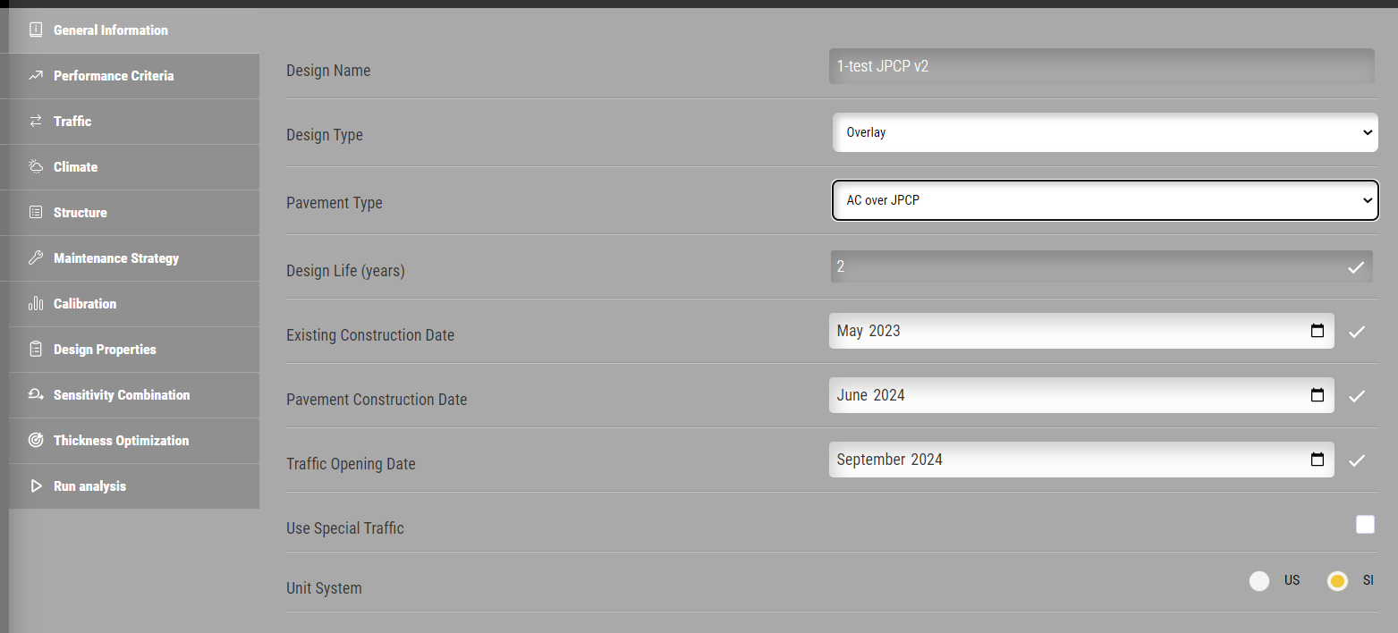
Figure 342: General Information

Populating the Inputs for this Interface

Design type: Select Overlay
Pavement type: Select AC over JPCP

In addition to selecting Design and Pavement type, select values for the following basic design parameters:

Design life (years): This control allows you to select from a list the period of time in years from AC overlay placement where the rehabilitated pavement is expected to perform adequately without significant loss of functional and structural integrity. Pavement performance is predicted over the design life beginning from the month the rehabilitated pavement is open to traffic.
Base construction: This control allows you to select the month and year when the construction of existing JPCP was completed.
Pavement construction: This control allows you to select the month and year when the AC overlay is scheduled to be placed.
Traffic opening: This control allows you to select the month and year the rehabilitated pavement is scheduled to be open to traffic. PMED predicts pavement performance beginning from this month and year.

Performance Criteria

Performance verification forms the basis of the acceptance or rejection of a trial rehabilitation design evaluated using PMED. The rehabilitation design procedure is based on pavement performance, and therefore, the critical levels of pavement distresses that can be tolerated by the agency at the selected level of reliability needs to be specified by the user. If the simulation process shows the trial design produces excessive amount of distresses, then the trial design must be modified accordingly to produce a feasible rehabilitation design in the future trials.

The distress types considered in the design of an AC overlay of existing JPCP are total rutting (all layers and subgrade), AC rutting, load-related top-down cracking (longitudinal cracking in the wheel path) and bottom-up fatigue cracking (alligator cracking), and thermal cracking (transverse cracking). Pavement smoothness is considered for performance verification and is characterized using the International Roughness Index (IRI). In addition, the transverse cracking of the existing JPCP and AC total cracking are also considered.

Figure 343: Performance Criteria

Populating the Inputs in this Interface

This table allows you to define the limits of critical distresses and smoothness that can be tolerated by the agency at the specified reliability levels. This table has three columns:

Performance Criteria: This column provides a list of performance indicators required to ensure that a pavement design will perform satisfactorily over its design life.
Limit: This column allows you to define the threshold values of these performance indicators to evaluate the adequacy of a design.
Reliability: This column allows you to define the probability at which the predicted distresses and smoothness will be less than the limits over the design period.

Note:
You can override the program defaults to enter project-specific threshold limits and reliability values representing agency policies. Refer to Chapter 8 of the AASHTO Manual of Practice for more guidance on selecting design criteria and reliability level.

Initial IRI (in./mile): The limit control allows you to define the expected smoothness immediately after the AC overlay is placed (expressed in terms of IRI). Initial IRI is a very important input as the time from AC overlay placement to attaining threshold IRI value is very much dependent on the initial IRI obtained at the time of rehabilitation. Thus, the initial IRI value provided must be what is typically attained in the field. You can override the PMED default value of 63 in./mi to reflect agency policy and guidelines.
Terminal IRI (in./mile): The limit and reliability controls for this criterion allow you to define the not-to-exceed limit for IRI at the end of the rehabilitation design life at a specified reliability level.
AC top-down fatigue cracking (% lane area): The limit and reliability controls for this criterion allow you to define the not-to-exceed limit for surface initiated fatigue cracking at the end of the rehabilitation design life at a specified reliability level.
AC bottom-up fatigue cracking (percent): The limit and reliability controls for this criterion controls allow you to define the not-to-exceed limit for bottom-initiated fatigue cracking at the end of the rehabilitation design life at a specified reliability level.
AC thermal cracking (ft./mile): The limit and reliability controls for this criterion allow you to define the not-to-exceed limit for non-load related transverse cracking at the end of the rehabilitation design life at a specified reliability level.
Permanent deformation - total pavement (in.): The limit and reliability controls for this criterion allow you to define the not-to-exceed limit for total rutting at the end of the rehabilitation design life at a specified reliability level. Total permanent deformation at the surface is the accumulation of the permanent deformation in all of the asphalt and unbound layers in the pavement system.
Permanent deformation - AC only (in.): The limit and reliability controls for this criterion allow you to define the not-to-exceed limit for rutting contributed by the AC layers at the end of the rehabilitation design life at a specified reliability level.
AC total cracking - bottom up + reflective (percent): The form of distress is only applicable to asphalt overlay pavements. The limit control allows you to define the not-to-exceed limit for AC total cracking at the end of the design life at 50 percent reliability level. The AC total cracking is the sum of bottom up fatigue cracking and reflective cracking that reflects from the existing layer through the HMA layer to the surface.
JPCP transverse cracking (percent slabs): The limit and reliability controls allow you to define the threshold value for transverse cracking of the existing JPCP at a user or agency specified reliability level. PMED predicts the combined percentage of PCC slabs with bottom-up and top-down transverse cracks that occurs mostly in the middle third of the slab. It is reported as percent slabs cracked.

Pavement Structure

This section explains adding additional layers to a pavement, editing the properties of those layers, and working with the pavement structure as a whole.

Asphalt Concrete

In PMED, the material types that fall under the following general definitions can be defined as an asphalt layer:

Hot Mix Asphalt (HMA)
Dense Graded
Open Graded Asphalt
Asphalt Stabilized Base Mixes
Sand Asphalt Mixtures
Stone Matrix Asphalt (SMA)
Cold Mix Asphalt
Central Plant Processed
Cold In-Place Recycling

If a small portion of asphalt and/or emulsion is added to granular base materials, and can be produced at a plant or mixed in-place, this material should not be considered as an AC layer. If needed, it should be combined with the crushed stone base materials or considered as an unbound aggregate mixture.

The key materials inputs required for asphalt concrete layers are:

Dynamic modulus of asphalt mixtures
Rheological properties of asphalt binder (e.g. viscosity, penetration, complex modulus and phase angles)
Creep compliance and indirect tensile strength
Mix related and other properties (e.g. effective binder content, air voids, heat capacity, thermal conductivity)
These inputs are required for predicting pavement responses, climatic analysis, asphalt aging as well as pavement performance.

Note:
For non-conventional mixtures, such as the Stone Matrix Asphalt or polymer-modified asphalt mixtures, it is recommended that you use laboratory-tested material properties. Levels 2 and 3 options for estimating dynamic modulus, indirect tensile strength and creep compliance properties provide reasonable results only for conventional Hot Mix Asphalt mixtures.

Interface

Figure 344: Asphalt Layer User Interface

Methods to Populate Inputs

There are two methods for entering data for the Asphalt Concrete layer:

Manual entry
Import from workspace library

Inputs

General Inputs

Thickness (inch, mm): This control allows you to define the thickness, in inches or millimeters, of the selected layer.

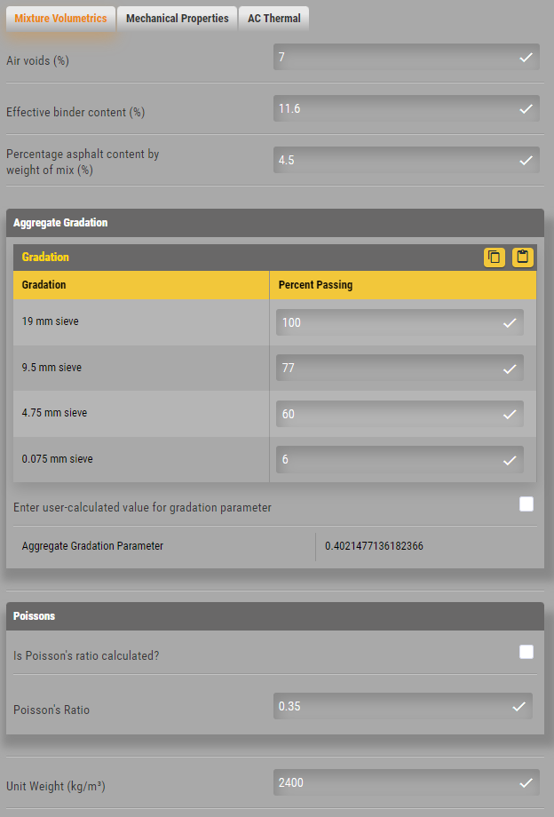
Mixture Volumetrics

Unit weight (\(lb/ft^3\), \(kg/m^3\)): This control allows you to define the weight of the selected material in pounds per cubic foot.
Effective binder content (%): This control allows you to define the effective binder content of the asphalt concrete mixture.
Air Voids (%): This control allows you to define the percent volume of air voids in the as-constructed asphalt concrete pavement layer.
Percent asphalt content by weight of mix (%): This control allows you to define the percent asphalt content by weight of mix (only used in the top-down cracking model). This input is only visible for the first asphalt layer in the user defined structure.
Aggregate Gradation:: This control allows you to enter the asphalt mixture gradation and calculates the aggregate parameter for the top-down cracking model. A user defined aggregate gradation parameter can also be entered.The required aggregate gradation inputs are:
- 3/4 inch (19 mm) sieve: This control allows you to define the cumulative amount of aggregate material (used in the asphalt mixture) that is passing on the 3/4 inch (19 mm) sieve.
- 3/8 inch (9.5 mm) sieve: This control allows you to define the cumulative amount of aggregate material (used in the asphalt mixture) that is passing on the 3/8 inch (9.5 mm) sieve.
- No. 4 (4.75 mm) sieve: This control allows you to define the cumulative amount of aggregate material (used in the asphalt mixture) that is passing on the #4 (4.75 mm) sieve.
- No. 200 (0.075 mm) sieve: This control allows you to define the amount of aggregate material (used in the asphalt mixture) that is passing on the #200 (0.075 mm) inch sieve.
Poisson’s ratio: This control allows you to define the Poisson’s ratio of the material in two ways: a constant value (Level 3) or calculate as a function of dynamic modulus (Level 2). Clicking the plus sign (+) to the left of this control presents the following options:
- Is Poisson’s ratio calculated?: Select True to calculate Poisson’s ratio as a function of dynamic modulus. Select False to use a constant value.
- Poisson’s ratio: This control allows you to define a constant value of Poisson’s ratio .This control is disabled when you select True.
- Poisson’s ratio Parameter A: This control allows you to define the parameter A of the Poisson’s ratio model. You can override the default value of -1.63 to enter mixture-specific values. This control is disabled when you select False.
- Poisson’s ratio Parameter B: This control allows you to define the parameter B of the Poisson’s ratio model. You can override the default value of 3.84E-06 to enter mixture-specific values. This control is disabled when you select False.

Note:
Parameters A and B are the empirical coefficients of the predictive model that defines Poisson’s ratio as a function of dynamic modulus, as described in the AASHTO Manual of Practice.

Mechanical Properties

Dynamic Modulus

Dynamic modulus input level: This control allows you to define the level of inputs for dynamic modulus of asphalt concrete material. Select one of the following options from the drop down menu:

Level 1: Selecting 1 gives you the option to input directly the laboratory tested dynamic modulus properties of the asphalt concrete mixture and laboratory tested asphalt binder properties.

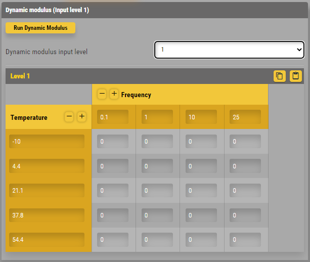
Figure 345: Dynamic Modulus Level 1

Select temperature level: This control allows you to define the number of test temperatures at which the dynamic modulus values is provided for a given mixture.
Select frequency level: This control allows you to define the number of test frequencies at which the dynamic modulus values is provided for a given mixture.

Note:
PMED allows a minimum of 3 and a maximum of 8 temperature levels. It also allows a minimum of 3 and a maximum of 6 frequency levels. Inputs at 5 temperature and 4 frequency levels are recommended.

Temperature (\(^\circ F\), \(^\circ C\)): This control allows you to define the temperature at which the dynamic modulus values were measured for a given mixture. You should enter at least one input value less than \(30^\circ F\) (\(-1^\circ C\)), another in the range of \(40\) to \(100^\circ F\) (\(4.44\) to \(37.78^\circ C\)), and the third input value higher than \(125^\circ F\) (\(51.67^\circ C\)).
Frequency (Hz): This control defines the test frequency at which the dynamic modulus values were measured for a given mixture. You should enter at least one input value less than 1 Hz, two in the range of 1-10 Hz and the fourth input value higher than 10 Hz.

You can populate the cells within the dynamic modulus table provided with corresponding dynamic modulus values for the user-defined temperature and frequency levels.

PMED provides the following default temperatures and frequencies:

US customary
- 14, 40, 70, 100 and 130 \(^\circ F\)
- 0.1, 1, 10 and 25 Hz.
SI
- -10, 4.44, 21.11, 37.78 and 54.54 \(^\circ C\)
- 0.1, 1, 10 and 25 Hz.

Level 2: Selecting 2 gives you the option to derive dynamic modulus properties from laboratory tested asphalt binder properties and the aggregate gradation of the asphalt concrete mixture.

Level 3: Selecting 3 gives you the option to derive dynamic modulus properties from typical rheological properties of the asphalt binder grade you select and the aggregate gradation of the asphalt concrete mixture.

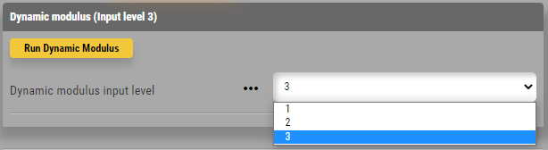
Figure 346: Dynamic Modulus Level 2 and 3

Note:
The model for determining frequency adjusted viscosity is research grade and not nationally calibrated, while the simple conversion model is nationally calibrated. This option is applicable only for Superpave binders at input levels 1 and 2.

Dynamic Modulus Predictive Model

Select HMA Estar predictive model: This control provides you the option for accounting the effects of loading frequencies when binder G* values are converted to viscosity values. Select True for frequency-adjusted viscosity estimates or False for simple conversion without frequency adjustments.

Reference Temperature

Reference temperature (\(^\circ F\), \(^\circ C\)): This control allows you to define a baseline temperature, in degrees Fahrenheit, for use in deriving the dynamic modulus mastercurve. The suggested value is \(70^\circ F\) (\(21.1^\circ C\).

Asphalt Binder Selection

Asphalt Binder: This control allows you to define the inputs of asphalt binder properties of asphalt concrete material. The controls in the drop down menu vary with the dynamic modulus input level you selected.

Note:
Once the dynamic modulus input level is selected, the program automatically defines the same input level for asphalt binder properties. Thus, a Level 1 dynamic modulus input selection will result in a Level 1 input selection for asphalt binder properties. Asphalt binder input level cannot be changed independent of the dynamic modulus input level.

Level 1:

SuperPave Performance Grade

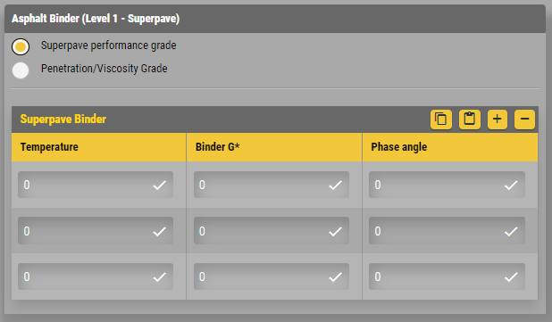
Figure 347: Level 1 SuperPave Performance

Temperature (\(^\circ F\), \(^\circ C\)): This control allows you to define the temperature at which the binder dynamic complex modulus, G*, and phase angle were measured for a given binder.
Binder G (Pascal):* This control allows you to define the complex shear modulus of the asphalt binder, measured at the test temperature given in the above control.
Phase angle (degree): This control allows you to define the phase angle measured at the given test temperature. You should enter at least three values in the above controls, though five is recommended.

Penetration or Viscosity Grade

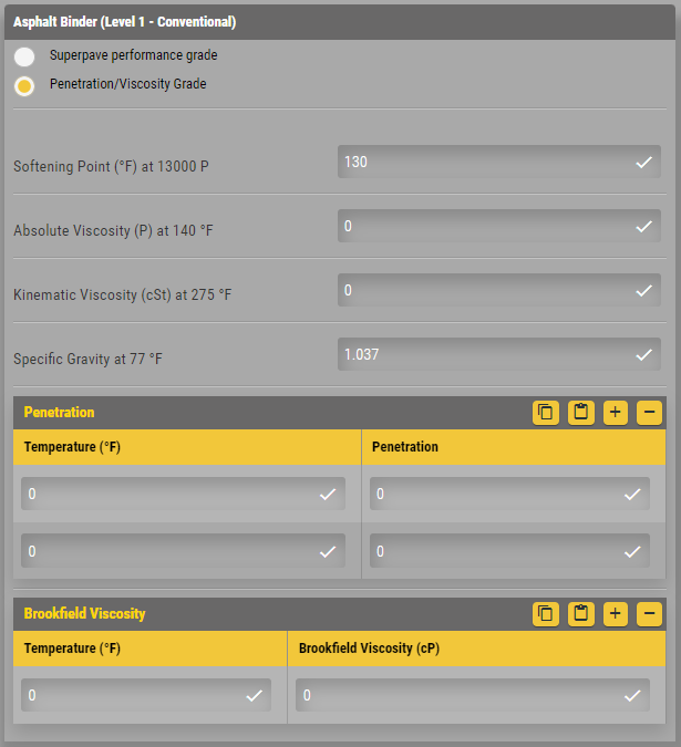
Figure 348: Level 1 Penetration and Viscosity

Softening point temperature at a viscosity of 13000 Poise: This control allows you to define the softening point temperature of the asphalt binder at a viscosity of 13000 Poise.
Absolute viscosity of the binder at 140 F: This control allows you to define the absolute viscosity of the asphalt binder at a temperature of 140°F.
Kinematic viscosity at 275 F in centistokes: This control allows you to define the kinematic viscosity of the asphalt binder at a temperature of 275°F.
Specific gravity of asphalt binder at 77 F: This control allows you to define the specific gravity of the asphalt binder at a temperature of 77°F.
Penetration (both temp and penetration value): This control allows you to define the both the temperature, in degrees Fahrenheit, and the corresponding penetration value of the asphalt binder.
Brookfield viscosity (both temp and viscosity): This control allows you to define the both the temperature, in degrees Fahrenheit, and the corresponding viscosity value of the asphalt binder.

You must enter values for the softening point, specific gravity, absolute viscosity, and kinematic viscosity of the asphalt binder as a minimum. In addition, you may choose to provide either binder penetration or Brookfield viscosity properties or both. PMED allows you to enter penetration or viscosity values for up to six test temperatures.

Level 3:

The user first selects a binder grading system (radio buttons) and then selects a binder grade from the dropdown menu. (Once a binder grade is selected, the program assumes and displays the typical values of A-VTS parameters for that binder grade).

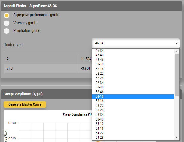
Figure 349: Level 3 SuperPave

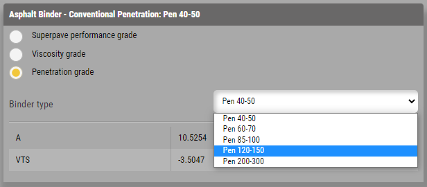
Figure 350: Level 3 Penetration

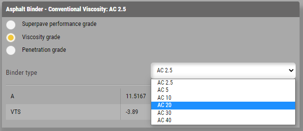
Figure 351: Level 3 Viscosity

Binder Grade Selection: This control allows you to define the binder grade type. Select one of the following options
- Superpave Performance Grade: This control allows you to select an appropriate PG binder from the options provided by the binder type dropdown menu.
- Viscosity Grade: This control allows you to select an appropriate viscosity- graded binder from the options provided by the binder type dropdown menu.
- Penetration Grade: This control allows you to select an appropriate penetration-graded binder from the options provided by the binder type dropdown menu.
- A: This control displays the intercept of the ASTM D2493 A-VTS relationship of the binder.
- VTS: This control displays the slope of the ASTM D2493 A-VTS relationship of the binder.

Indirect tensile strength at 14 deg F: Indirect tensile strength at -10 deg C: This control allows you to define the indirect tensile strength of the asphalt concrete mixture at a temperature of -10˚C. You can enter a laboratory measured value (Levels 1 and 2) or allow the program to calculate a typical value (Level 3) based on statistical relationships with other AC inputs.

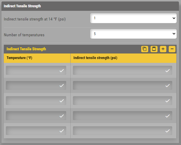
Figure 352: Level 1 IDT

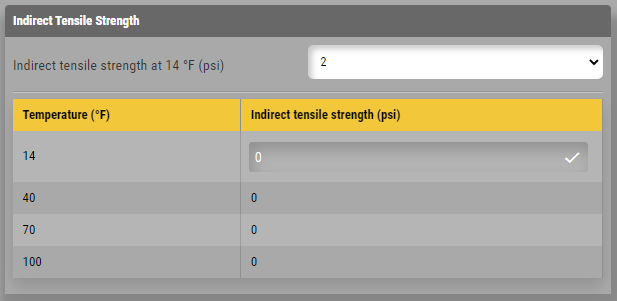
Figure 353: Level 2 IDT

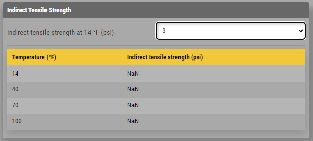
Figure 354: Level 3 IDT

Thermal

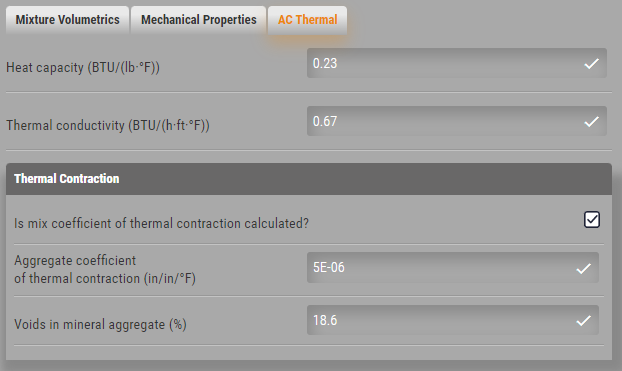
Figure 355: Asphalt Thermal

Thermal conductivity (BTU/hr-ft-deg F): This control allows you to define the thermal conductivity of the asphalt concrete material. PMED provides a default value of 0.67.
Heat capacity (BTU/lb-deg F): This control allows you to define the heat capacity of the asphalt concrete material. PMED provides a default value of 0.23.
Thermal contraction: This control allows you to define the coefficient of thermal contraction of the AC mix in two ways: a direct entry of the coefficient or allow the program to compute as a function of thermal contraction coefficient of the aggregates. Clicking the sign () to the left of this control presents the following options:
Is thermal contraction calculated?: Select True to calculate the mix contraction coefficient as a function of the aggregate contraction coefficient. Select False to directly enter the mix contraction coefficient.
Mix coefficient of thermal contraction: This control allows you to directly enter the coefficient of thermal contraction of the AC mix. PMED provides a default value of 1.3E-05 in./in./˚F.
Aggregate coefficient of thermal contraction: This control allows you to directly input the coefficient of thermal contraction of the aggregates. PMED provides a default value of 5.0 E-06 in./in./˚F.

PCC (Existing Intact JPCP) Layer

Interface

Figure 356: PCC Inputs

Methods to Populate Inputs

There are two methods for entering data for the Portland Cement Concrete layer:

Manual entry
Import from workspace library

Inputs

PCC

Thickness (in.): This control allows you to define the thickness of the PCC layer used in the trial design. Note that this input has a significant impact on PMED prediction of future JPCP performance.
Unit weight (pcf): This control allows you to define the weight per unit volume of the PCC mix design. Typical values ranges from 140 to 160 pcf.
Poisson’s ratio: This control allows you to define the PCC’s Poisson’s ratio (defined as the ratio of PCC lateral and longitudinal strain under applied loading). Poisson’s ratio is an important input required for structural analysis. Values between 0.15 and 0.18 are typical PCC used in JPCP construction.

Thermal

PCC coefficient of thermal expansion (in/in/deg F x 10-6): This control allows you to define the expansion or contraction a material undergoes with change in temperature. PCC coefficient of thermal expansion (CTE) is defined as the increase in length per unit length of PCC (typically 1-in) for a unit increase in temperature (typically 1 ˚F). PCC CTE has a significant impact on critical curling stresses developed in the JPCP PCC slab and thus the development of transverse cracks. PCC CTE can be considered to be a very critical input that influences the development of transverse cracking.
PCC thermal conductivity (BTU/hr-ft-deg F): This control allows you to define the ability of the PCC material to uniformly conduct heat through its thickness when subjected to a temperature differential at the top surface and bottom of the PCC layer. PMED provides a typical value of 1.25 BTU/hr-ft-˚F.
PCC heat capacity (BTU/lb-deg F): This control allows you to define the amount of heat required to raise a unit mass of PCC material (typically 1 Ib) by a unit temperature (typically 1 ˚F). PMED provides a typical value of 0.28 BTU/hr-ft-deg F.

Note:
The CTE should be adjusted as follows to reflect the CTE values used to calibrate the current models . CTE input =CTEpcc – CTEcalib + 9.6110-6 in/in/ ˚F CTEinput = CTE adjusted to reflect CTE values used in calibration, in/in/ ˚F CTEpcc = CTE of concrete specimen according to AASHTO T 336 or TP 60, in/in/ ˚F CTEcalib = CTE of 304 stainless steel calibration or verification specimen used to determine CTEpcc, in/in/ ˚F CTE values contained in the LTPP Standard Data Release 24.0 dated January 2010 or later have been updated with this correction. These CTE values should be increased by 0.8310-6 in/in/ ˚F if they are used as a level 3 input. CTE values prior to LTPP SDR 24.0 do not need to be adjusted.

Mix

-Cement type: This control allows you to select the type of cement used in the PCC mix. PMED allows you to select one of the following Portland cement types: - Type I: Type I cements are described as general purpose cements suitable for most pavement construction situations where special properties such as high early strength, high durability, etc., are not required. - Type II: Type II cements contain no more than 8% tricalcium aluminate (C3A) and are suitable for situations where moderate sulfate resistance is required. - Type III: Type III cements have constituents very similar to Type I cements. However, the constituents are ground to produce a finer mix that produces higher levels of early strengths. Thus, Type II cements are generally used in JPCP construction where early strength is required.

Note:
For PCC mixes with non-conventional cement types, select the cement type provided by PMED which is closest in characteristics.

-Cementitious material content (lb/yd3): This control allows you to define the total weight of cementitious material (portland cement, pozzolans, lime, fly-ash, etc.) per unit volume of PCC as per the PCC mix design. The cementitious material along with water content is used to calculate PCC ultimate shrinkage, a critical parameter in structural analysis.

Water to cement ratio: This control allows you to define the ratio of the weight of water to the weight of all cementitious materials used in the PCC mix design. This input is used to calculate the water content of the PCC mix and is used along with cementitious material content to calculate PCC ultimate shrinkage, a critical parameter in structural analysis.
Aggregate type: This control allows you to select the coarse aggregate rock type in the PCC mix. If the coarse aggregate rock type is not uniform, the predominant rock type must be selected. Coarse aggregate is typically described as the material the material retained on the No. 4 sieve. Coarse aggregate rock type is used to calculate PCC ultimate shrinkage. PMED allows you select one of the following coarse aggregate rock types:
Quartzite: This option allows you to select quartzite as the predominant coarse aggregate rock type in the PCC mix. Quartzite is a metamorphic rock which is extremely resistant to weathering and erosion.
Limestone: This option allows you to select limestone as the predominant coarse aggregate rock type in the PCC mix. Limestone is a sedimentary rock composed largely calcium carbonate and provides a solid base for highway pavements.
Dolomite: This option allows you to select dolomite as the predominant coarse aggregate rock type in the PCC mix. Dolomite is a sedimentary carbonate rock composed mainly of calcium magnesium carbonate. Dolomite like limestone provides a solid base for highway pavements.
Granite: This option allows you to select granite as the predominant coarse aggregate rock type in the PCC mix. Granite is an intrusive, felsic, igneous rock and is extremely resistant to weathering and erosion.
Rhyolite: This option allows you to select rhyolite as the predominant coarse aggregate rock type in the PCC mix. Rhyolite is an igneous, volcanic (extrusive) rock and is extremely resistant to weathering and erosion.
Basalt: This option allows you to select basalt as the predominant coarse aggregate rock type in the PCC mix. Basalt is an extrusive igneous rock and is extremely resistant to weathering and erosion.
Syenite: This option allows you to select syenite as the predominant coarse aggregate rock type in the PCC mix. Syenite is a coarse-grained intrusive igneous rock of the same general composition as granite but with the quartz either absent or present in relatively small amounts. Syenite is extremely resistant to weathering and erosion.
Gabbro: This option allows you to select gabbro as the predominant coarse aggregate rock type in the PCC mix. Gabbro is an intrusive mafic igneous rock, rich in iron and magnesium, poor in silica (quartz) and chemically equivalent to basalt. Gabbro is extremely resistant to weathering and erosion.
Chert: This option allows you to select chert as the predominant coarse aggregate rock type in the PCC mix. Chert is a sedimentary rock widely used in highway pavement construction. It is moderately resistant to weathering and erosion.
PCC set temperature (deg F): This control allows you to define the PCC temperature when the freshly placed PCC slab becomes solid. PCC set temperature can be user entered or estimated by PMED using (1) average of hourly ambient temperatures for month of construction and (2) cementitious material content. The default for this control is to let PMED calculate the PCC set temperature. You can, however, override the PMED default and enter your own PCC set temperature.
Calculated internally? This control allows you to decide whether PMED should calculate PCC set temperature or not by selecting one of the following options:
True: Selecting this option allows PMED to calculate the PCC set temperature.
False: This option allows you to input directly PCC set temperature.
User-specified PCC set temperature: This control allows you define the PCC set temperature in degrees Fahrenheit (minimum 70, maximum 212).
Ultimate shrinkage (microstrain): This control allows you to define the ultimate (long-term) shrinkage strain that PCC will develop under laboratory controlled conditions of temperature and humidity (e.g., 40% relative humidity). The default for this control is to let PMED calculate PCC ultimate shrinkage internally. You can, however, override the PMED default and enter your own PCC ultimate shrinkage.
Calculated internally? This control allows you to decide whether PMED should calculate PCC ultimate shrinkage or not by selecting one of the following options:
True: Selecting this option allows PMED to calculate the PCC ultimate shrinkage.
False: This option allows you to input directly PCC ultimate shrinkage.
User-specified PCC ultimate shrinkage: This control allows you define the PCC ultimate shrinkage in microstrain (minimum 300, maximum 1000).
Reversible Shrinkage (%): Change in PCC humidity/moisture affects the volume of PCC with moisture causes PCC expansion while drying causes PCC shrinkage. Note that this is very different from the drying shrinkage in PCC due to moisture loss during PCC hardening that result in irreversible shrinkage. This control allows you to define the percent of PCC ultimate shrinkage that can be recovered due to changes in PCC humidity/moisture (minimum 0, maximum 100).
Time to develop 50% of ultimate shrinkage (days): This control allows you to define the time required in days to develop 50% of PCC ultimate shrinkage (minimum 30, maximum 50).
Curing method: This control allows you to select curing method applied after PCC placement. PMED allows you to select one of the following options:
Wet Curing: These are curing methods that prevent PCC surface moisture loss by supplying additional water to the PCC surface. The most common practice is to place wet burlap or other natural or synthetic-fiber blankets at the PCC surface to prevent rapid evaporation of moisture. Selecting this option implies the use of the above listed methods or similar techniques for PCC curing.
Curing Compound: These are curing methods that prevent moisture loss at the PCC surface by placing a liquid membrane-forming chemical compound (typically resins, waxes or synthetic rubbers dissolved in a solvent) that forms a near-impermeable membrane over the PCC once the solvent evaporates. Selecting this option implies the use of the above listed methods or similar techniques for PCC curing.

Strength

PMED requires both PCC modulus of rupture and elastic modulus.

PCC strength input level: This control allows you to select modulus of rupture and elastic modulus input level. PMED allows for the following options:
Level 1: This option allows you to directly input the 7-, 14-, 28-, and 90-day PCC elastic modulus and modulus of rupture. For this option, the 20-yr and 28-day PCC elastic modulus and modulus of rupture ratios are also required.
Level 2: This option allows you to directly input the 7-, 14-, 28-, and 90-day PCC compressive strength. For this option, the 20-yr and 28-day PCC compressive strength ratio is also required.
Level 3: This option allows you to directly input any of the following combination of inputs:
28-day PCC modulus of rupture only.
28-day PCC compressive strength only.
28-day PCC modulus of rupture and 28-day PCC elastic modulus.
28-day PCC compressive strength and 28-day PCC elastic modulus.
Level 1 Modulus of Rupture/Elastic Modulus Table: This table allows you to define modulus of rupture and elastic modulus of the existing PCC layer:
Time: This column lists the age of the existing PCC layer at which the AC overlay is placed. The age is computed internally by PMED using the existing construction date and pavement (rehabilitation) construction date.
Modulus of Rupture (psi): This column allows you to define PCC modulus of rupture of the existing PCC layer.
Elastic Modulus (psi): This column allows you to define the elastic modulus of the existing PCC layer. The backcalculated “dynamic” elastic modulus values must be adjusted to “static” values. Refer to the AASHTO Manual of Practice for guidance.
User-defined Modulus Adjustment Factor: This control allows you enter an adjustment factor to convert backcalculated dynamic modulus to static modulus.

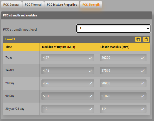
Figure 357: PCC Strength 1

Level 2 Compressive Strength Table: This table allows you to define the compressive strength of the existing PCC layer:
Time: This column lists the age of the existing PCC layer at which the AC overlay is placed. The age is computed internally by PMED using the existing construction date and pavement (rehabilitation) construction date.
Compressive strength (psi): This column allows you to define the compressive strength of the existing PCC layer.

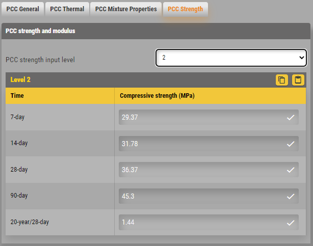
Figure 358: PCC Strength 2

Level 3 Modulus of Rupture, Compressive Strength, and Elastic Modulus Table: This control allows you to define your preferred combination of PCC strength and elastic modulus inputs at Level 3. PMED allows for the following combination of inputs by checking the appropriate radio button and check box:
28-day PCC modulus of rupture only.
28-day PCC compressive strength only.
28-day PCC modulus of rupture and 28-day PCC elastic modulus.
28-day PCC compressive strength and 28-day PCC elastic modulus.

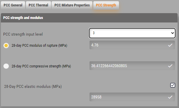
Figure 359: PCC Strength 3

Asphalt Concrete Base Layer

Interface

Figure 360: Asphalt Layer User Interface

Methods to Populate Inputs

There are two methods for entering data for the Asphalt Concrete layer:

Manual entry
Import from workspace library

Inputs

Asphalt

Thickness (in): This control allows you to define the thickness, in inches, of the selected layer.

Mixture Volumetrics

Unit weight (pcf): This control allows you to define the weight of the selected material in pounds per cubic foot.
Effective binder content (%): This control allows you to define the effective binder content of the asphalt concrete mixture.
Air Voids (%): This control allows you to define the percent volume of air voids in the as-constructed asphalt concrete pavement layer.
Poisson’s ratio: This control allows you to define the Poisson’s ratio of the material in two ways: a constant value (Level 3) or calculate as a function of dynamic modulus (Level 2). Clicking the plus sign (+) to the left of this control presents the following options:
Is Poisson’s ratio calculated?: Select True to calculate Poisson’s ratio as a function of dynamic modulus. Select False to use a constant value.
Poisson’s ratio: This control allows you to define a constant value of Poisson’s ratio .This control is disabled when you select True.
Poisson’s ratio Parameter A: This control allows you to define the parameter A of the Poisson’s ratio model. You can override the default value of -1.63 to enter mixture-specific values. This control is disabled when you select False.
Poisson’s ratio Parameter B: This control allows you to define the parameter B of the Poisson’s ratio model. You can override the default value of 3.84E-06 to enter mixture-specific values. This control is disabled when you select False.

Note:
Parameters A and B are the empirical coefficients of the predictive model that defines Poisson’s ratio as a function of dynamic modulus, as described in the AASHTO Manual of Practice.

Mechanical Properties

Dynamic modulus input level: This control allows you to define the level of inputs for dynamic modulus of asphalt concrete material. Select one of the following options from the dropdown menu:
Level 1: Selecting 1 gives you the option to input directly the laboratory tested dynamic modulus properties of the asphalt concrete mixture and laboratory tested asphalt binder properties. These are described in the AASHTO Manual of Practice as Level 1 inputs.
Level 2: Selecting 2 gives you the option to derive dynamic modulus properties from laboratory tested asphalt binder properties and the aggregate gradation of the asphalt concrete mixture. These are described in the AASHTO Manual of Practice as Level 2 inputs.
Level 3: Selecting 3 gives you the option to derive dynamic modulus properties from typical rheological properties of the asphalt binder grade you select and the aggregate gradation of the asphalt concrete mixture. These are described in the AASHTO Manual of Practice as Level 3 inputs.

Note:
Input screens for dynamic modulus and AC binder properties change with the input level selected. For example, the input screen for dynamic modulus properties at level 1 is different from those at levels 2 and 3, while for asphalt binder properties, the input screens at levels 1 and 2 are different from that of Level 3.

Dynamic Modulus

Dynamic Modulus Input Level 1

This control allows you to define the Level 1 dynamic modulus values of the asphalt concrete mixture.

Figure 361: Dynamic Modulus Level 1

Select temperature level: This control allows you to define the number of test temperatures at which the dynamic modulus values is provided for a given mixture.
Select frequency level: This control allows you to define the number of test frequencies at which the dynamic modulus values is provided for a given mixture.
Temperature (deg F): This control allows you to define the temperature at which the dynamic modulus values were measured for a given mixture. You should enter at least one input value less than 30˚F, another in the range of 40 to 100˚F, and the third input value higher than 125˚F.
Frequency (Hz): This control defines the test frequency at which the dynamic modulus values were measured for a given mixture. You should enter at least one input value less than 1 Hz, two in the range of 1-10 Hz and the fourth input value higher than 10 Hz.

You can populate the cells within the dynamic modulus table provided with corresponding dynamic modulus values for the user-defined temperature and frequency levels. PMED provides default temperatures of 14, 40, 70, 100 and 130˚F, and default frequencies of 0.1, 1, 10 and 25 Hz.

Note:
Input screens for dynamic modulus and AC binder properties change with the input level selected. For example, the input screen for dynamic modulus properties at level 1 is different from those at levels 2 and 3, while for asphalt binder properties, the input screens at levels 1 and 2 are different from that of Level 3.

Right-Click Menu Options

Right-click on a cell in the dynamic modulus table to access the following functionality:

Copy: This menu item copies the selected value.
Paste: This menu item pastes the copied value.
Import MEPDG Dynamic Modulus (.dwn) Format: This menu item allows you to import a dynamic modulus file that was created in using MEPDG.

Dynamic Modulus Input Levels 2 and 3

This control allows you to define the aggregate gradation of the asphalt concrete mixture for use in dynamic modulus calculations.

Figure 362: Dynamic Modulus Level 2 and 3

3/4-inch sieve: This control allows you to define the cumulative amount of aggregate material (used in the asphalt mixture) that is passing on the ¾ inch sieve.
3/8-inch sieve: This control allows you to define the cumulative amount of aggregate material (used in the asphalt mixture) that is passing on the 3/8 inch sieve.
No. 4 sieve: This control allows you to define the cumulative amount of aggregate material (used in the asphalt mixture) that is passing on the #4 sieve.
No. 200 sieve: This control allows you to define the amount of aggregate material (used in the asphalt mixture) that is passing on the #200 inch sieve.

Note:
The model for determining frequency adjusted viscosity is research grade and not nationally calibrated, while the simple conversion model is nationally calibrated. This option is applicable only for Superpave binders at input levels 1 and 2.

Select HMA Estar Predictive Model

Select HMA Estar predictive model: This control provides you the option for accounting the effects of loading frequencies when binder G* values are converted to viscosity values. Select True for frequency-adjusted viscosity estimates or False for simple conversion without frequency adjustments.

Reference Temperature

Reference temperature (deg F): This control allows you to define a baseline temperature, in degrees Fahrenheit, for use in deriving the dynamic modulus mastercurve. The suggested value is 70˚F.

Asphalt Binder

Asphalt Binder: This control allows you to define the inputs of asphalt binder properties of asphalt concrete material. The controls in the dropdown menu vary with the dynamic modulus input level you selected.

Note:
Once the dynamic modulus input level is selected, the program automatically defines the same input level for asphalt binder properties. Thus, a Level 1 dynamic modulus input selection will result in a Level 1 input selection for asphalt binder properties. Asphalt binder input level cannot be changed independent of the dynamic modulus input level.

Asphalt Binder Levels 1 and 2

You must first select an appropriate binder grading system and then enter the binder properties.

Superpave Performance Grade

Figure 363: Level 1 SuperPave Performance

Temperature (deg F): This control allows you to define the temperature at which the binder dynamic complex modulus, G*, and phase angle were measured for a given binder.
**Binder G*:** This control allows you to define the complex shear modulus of the asphalt binder, measured at the test temperature given in the above control.
Phase angle: This control allows you to define the phase angle measured at the given test temperature.

You should enter at least three values in the above controls, though five is recommended.

Right-Click Menu Options

Right-click on a cell in the table to access the following functionality:

Copy: This menu item copies the selected value.
Paste: This menu item pastes the copied value.
Import MEPDG Binder (.bif) Format: This menu item allows you to import a binder modulus file that was created in using MEPDG.

Penetration/Viscosity Grade

Figure 364: Level 1 Penetration and Viscosity

Softening point temperature at a viscosity of 13000 Poise: This control allows you to define the softening point temperature of the asphalt binder at a viscosity of 13000 Poise.
Absolute viscosity of the binder at 140 F: This control allows you to define the absolute viscosity of the asphalt binder at a temperature of 140˚F.
Kinematic viscosity at 275 F in centistokes: This control allows you to define the kinematic viscosity of the asphalt binder at a temperature of 275˚F.
Specific gravity of asphalt binder at 77 F: This control allows you to define the specific gravity of the asphalt binder at a temperature of 77˚F.
Penetration (both temp and penetration value): This control allows you to define the both the temperature, in degrees Fahrenheit, and the corresponding penetration value of the asphalt binder.
Brookfield viscosity (both temp and viscosity): This control allows you to define the both the temperature, in degrees Fahrenheit, and the corresponding viscosity value of the asphalt binder.

Asphalt Binder Level 3

Figure 365: Level 3 SuperPave

Figure 366: Level 3 Penetration

Figure 367: Level 3 Viscosity

Grade: These controls allow you to define the grade of the binder. Select one of the following options:
Superpave Performance Grade: This control allows you to select an appropriate PG binder from the options provided by the binder type dropdown menu.
Viscosity Grade: This control allows you to select an appropriate viscosity-graded binder from the options provided by the binder type dropdown menu.
Penetration Grade: This control allows you to select an appropriate penetration-graded binder from the options provided by the binder type dropdown menu.
- A: This control displays the intercept of the ASTM D2493 A-VTS relationship of the binder.
- VTS: This control displays the slope of the ASTM D2493 A-VTS relationship of the binder.

Indirect Tensile Strength at 14 deg F

PMED does not require indirect tensile strength for an asphalt concrete base layer. Although the defaults of these inputs may be displayed, PMED does not use them in calculations.

Creep Compliance

PMED does not require creep compliance inputs for an asphalt concrete base layer. Although the defaults of these inputs may be displayed, PMED does not use them in calculations.

Thermal Properties

Thermal conductivity (BTU/hr-ft-deg F): This control allows you to define the thermal conductivity of the asphalt concrete material. PMED provides a default value of 0.67.
Heat capacity (BTU/lb-deg F): This control allows you to define the heat capacity of the asphalt concrete material. PMED provides a default value of 0.23.

Figure 368: Asphalt Thermal

Note:
PMED does not require mix coefficient of thermal contraction inputs for an asphalt concrete base layer. Although the defaults of these inputs may be displayed, PMED does not use them in calculations

Chemically Stabilized Layer

The required inputs for a chemically stabilized layer can be broadly classified as general, strength, and thermal properties. Note that the strength properties required by PMED are different for flexible and rigid pavements.

The chemically stabilized materials include lean concrete, cement stabilized, open graded cement stabilized, soil cement, lime-cement-flyash, and lime treated materials.

You can use the following guidance to decide when a level of material stabilization is adequate to be considered as a chemically stabilized layer or not:

Chemically stabilized materials that are “engineered” to provide long-term strength and durability should be considered as a chemically stabilized layer (e.g. cement treated, lean concrete, pozzolonic treated). Typically such layers are placed directly under the lowest asphalt layer.
Lime and/or lime-fly ash stabilized soils could be considered a chemically stabilized layer, if these layers are engineered to provide structural support and have a sufficient amount of stabilizer mixed in with the soil.
Lime and/or lime-fly ash stabilized soils could be also considered as a material layer that is insensitive to moisture and the resilient modulus or stiffness of these layers can be held constant over time.
Aggregate or granular base materials treated with small amounts of chemical stabilizers to enhance constructability (e.g. lower the plasticity index, improve the strength) should not be considered as a chemically stabilized layer. They should be considered as an unbound material, and combined with those unbound layers, if necessary (e.g. soil cement). Typically such layers are placed deeper in the pavement structure.

Interface

Figure 369: Chemically Stabilized Layer

Methods to Populate Inputs

There are three methods for entering data for the Stabilized (Flexible) layer:

Manual entry
Import from workspace library

Inputs

General Inputs

Layer thickness (inch,mm): This control allows you to define the thickness of the stabilized base layer.
Poisson’s ratio: This control allows you to define the Poisson’s ratio of the chemically stabilized material. Values between 0.15 and 0.35 are typical for chemically stabilized materials.
Unit weight (\(lb/ft^3\), \(kg/m^3\)): This control allows you to define the weight per unit volume of the stabilized base material. PMED provides a default value of 150 pcf.

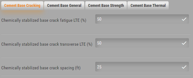
Strength Properties

Elastic/resilient modulus (psi): This control allows you to define the required elastic/ resilient modulus value of chemically stabilized materials.
Minimum elastic/resilient modulus (psi): This control allows you to define the minimum modulus of chemically stabilized material that represents deteriorated condition under increased levels of fatigue damage. This input is required only for flexible pavements with a chemically stabilized layer placed directly under the AC layer. PMED will not display this control for other pavement types.
Modulus of Rupture (psi): This control allows you to define the modulus of rupture of chemically stabilized material. The 28-day value is used for design. This input is required only for flexible pavements with a chemically stabilized layer placed directly under the AC layer. PMED will not display this control for other pavement types.

Note:
These inputs can be determined either through laboratory testing, correlations, or based on agency experience and historical records for levels 1, 2 and 3, respectively.

Thermal Properties

Thermal conductivity (BTU/hr-ft-deg F): This control allows you to define the thermal conductivity of the chemically stabilized material. PMED provides a default value of 1.25 Btu/(ft)(hr)(˚F).
Heat capacity (BTU/lb-deg F): This control allows you to define the heat capacity of the chemically stabilized material. PMED provides a default value of 0.28 Btu/(lb)(˚F).

Non-stabilized unbound base

Non-stabilized materials include AASHTO soil classes A-1 through A-3, as well as those commonly defined in practice as crushed stone, crushed gravel, river gravel, permeable aggregate, and cold recycled asphalt material (includes millings and in-place pulverized material).

Inputs required for non-stabilized materials include physical and engineering properties such as dry density, moisture content, hydraulic conductivity, specific gravity, soil-water characteristic curve (SWCC) parameters, classification properties, and the resilient modulus.

Interface

Figure 370: Unbound

Methods to Populate Inputs

There are two methods for entering data: - Manual entry - Import from workspace library

Inputs

General Inputs

Layer thickness (in, mm): This control allows you to define the thickness of the selected layer.
Poisson’s ratio: This control allows you to define the Poisson’s ratio of the unbound material. PMED provides a default value of 0.35.
Coefficient of lateral earth pressure (k0): This control allows you to define the pressure that the unbound material exerts in the horizontal plane. PMED provides a default value of 0.5.

Resilient Modulus

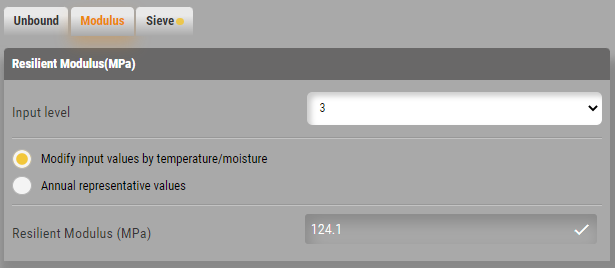
Resilient Modulus (psi, MPa): This control allows you to define the level of inputs for resilient modulus of the unbound material. This control also allows you to define the resilient modulus or the other material properties that correlate with the resilient modulus. PMED displays the default value (Level 3) for the selected material class. Click on the Resilient Modulus control to modify the default value and/or input level.

Input Level: This control allows you to define the level of inputs for the non-stabilized material. You can select one of the following options:
- Level 1: PMED does not provide Level 1 inputs option for resilient modulus of non-stabilized materials.
- Level 2: This option allows you to define the resilient modulus directly or using its correlations with soil index and strength properties. This level of input is considered as Level 2 in the AASHTO Manual of Practice.
- Level 3: This option allows you to override the default resilient modulus value (Level 3) of the non-stabilized material.
Analysis Types: These controls allow you to define how PMED accounts for seasonal variations (freezing, thawing and moisture) in the resilient modulus calculations. Select one of the following options:
- Modify input values by temperature/moisture: This option allows you to define a single resilient modulus value. You can also input a single value of the selected soil index or strength property that is converted by PMED into a resilient modulus value. PMED incorporates the effects of seasonal variations on the single resilient modulus value you define.
- Monthly representative values: This option allows you to define the resilient modulus throughout the year. You can input a single value of resilient modulus (or the selected soil index or strength property) for each month of a year. By selecting this option, you make PMED use the inputs you provide directly for seasonal variations without making internal adjustments. This option is available only for Level 2 inputs.
- Annual representative values: This option allows you to define a fixed resilient modulus for an entire year. You can input a single value of resilient modulus (or the selected soil index or strength property) that is representative for an entire year. PMED does not incorporate the effects of seasonal variations on the single resilient modulus value you define.
Correlation Methods to estimate Resilient Modulus: This control allows you to select how to estimate the resilient modulus using one of the following options:
- Resilient modulus (psi, MPa)
- California Bearing Ratio (CBR) (percent) R-value
- Layer Coefficient-ai
- Dynamic Cone Penetrometer (DCP) Penetration (in./blow, mm/blow)
- Plasticity Index (PI) and Gradation (i.e., Percent Passing No. 200 (0.075mm) sieve)
Input Entry Table: This control allows you to define the values for resilient modulus or the selected soil index and strength property.

Aggregate Gradation and other engineering properties

The aggregate gradation dialog box allows you to define the particle size distribution, Atterberg limits, specific gravity, water content, maximum dry density, saturated hydraulic conductivity and the SWCC parameters of non-stabilized materials. A description of the available inputs are summarized below.

Sieve Size Table: This table allows you to define the percentage of non-stabilized material passing a variety of sieve sizes.
- Sieve Opening Size (in, mm): This column lists the applicable sieve sizes.
- Percent Passing: This column allows you to define the percentage of non-stabilized material passing a given sieve size. You are not required to define the percent passing for each sieve size. However, you are required to enter values for a minimum of 3 sieve sizes including No. 200 sieve.
- Liquid Limit This control allows you to define the liquid limit of the non-stabilized material.
- Plasticity Index: This control allows you to define the plasticity index for non-stabilized material.
- Is Layer Compacted?: Enable this control to indicate that the layer is compacted. Typically non-stabilized materials used in the base and subbase layers are compacted in place during construction. Disable this control to indicate that the layer is not compacted.
- Maximum dry unit weight (\(lb/ft^3\), \(kg/m^3\)): PMED internally computes the maximum dry unit weight of the non-stabilized material. This control allows you to override the internally computed value by enabling the check box. Click the check box to enable/disable this control.
- Saturated hydraulic conductivity (ft/hr, m/hr): PMED internally computes the saturated hydraulic conductivity of the non-stabilized material. This control allows you to override the internally computed value by enabling the check box. Click the check box to enable/disable this control.
- Specific gravity of solids: PMED internally computes the specific gravity of the non-stabilized material. This control allows you to override the internally computed value by enabling the check box. Click the check box to enable/disable this control.
- Optimum gravimetric water content (%): PMED internally computes the moisture content of the non-stabilized material at which maximum dry density is achieved. This control allows you to override the internally computed value by enabling the check box. Click the check box to enable/disable this control.
- User-defined Soil Water Characteristic Curve (SWCC): PMED internally computes the coefficients (af, bf, cf, and hr) of the soil water characteristic curve. This control allows you to override the internally computed value by enabling the check box. Click the check box to enable/disable this control.

Note:
PMED internally computes the values of the following properties based on the inputs for Gradation, Liquid Limit, Plasticity Index and Is Layer Compacted. The computed values are based on the defaults initially displayed on the input screen. However, if you choose to modify the default values, you are required to click outside the input screen for the program to update the internally computed values.

Note:
Input compatibility: It is essential that the values entered for water content, maximum dry unit weight are compatible. If the value water content entered represents optimium conditions, then the maximum dry unit weight at optimum conditions should also be entered.

Subgrade

Subgrade materials include AASHTO soil classes A-1 through A-3, as well as those commonly defined in practice as crushed stone, crushed gravel, river gravel, permeable aggregate, and cold recycled asphalt material (includes millings and in-place pulverized material).

Inputs required for subgrade materials include physical and engineering properties such as dry density, moisture content, hydraulic conductivity, specific gravity, soil-water characteristic curve (SWCC) parameters, classification properties, and the resilient modulus.

Interface

Figure 371: Subgrade

Methods to Populate Inputs

There are two methods for entering data: - Manual entry - Import from workspace library

Inputs

General Inputs

Layer thickness (in, mm): This control allows you to define the thickness of the selected layer.
Poisson’s ratio: This control allows you to define the Poisson’s ratio of the subgrade material. PMED provides a default value of 0.35.
Coefficient of lateral earth pressure (k0): This control allows you to define the pressure that the unbound material exerts in the horizontal plane. PMED provides a default value of 0.5.

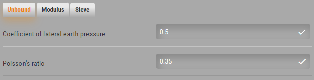
Figure 372: Subgrade Unbound

Resilient Modulus

Input Level: This control allows you to define the level of inputs for the subgrade material. You can select one of the following options:
- Level 1: PMED does not provide Level 1 inputs option for resilient modulus of subgrade materials.
- Level 2: This option allows you to define the resilient modulus directly or using its correlations with soil index and strength properties. This level of input is considered as Level 2 in the AASHTO Manual of Practice.
- Level 3: This option allows you to override the default resilient modulus value (Level 3) of the subgrade material.
Analysis Types: These controls allow you to define how PMED accounts for seasonal variations (freezing, thawing and moisture) in the resilient modulus calculations. Select one of the following options: -Modify input values by temperature/moisture: This option allows you to define a single resilient modulus value. You can also input a single value of the selected soil index or strength property that is converted by PMED into a resilient modulus value. PMED incorporates the effects of seasonal variations on the single resilient modulus value you define. -Monthly representative values: This option allows you to define the resilient modulus throughout the year. You can input a single value of resilient modulus (or the selected soil index or strength property) for each month of a year. By selecting this option, you make PMED use the inputs you provide directly for seasonal variations without making internal adjustments. This option is available only for Level 2 inputs. -Annual representative values: This option allows you to define a fixed resilient modulus for an entire year. You can input a single value of resilient modulus (or the selected soil index or strength property) that is representative for an entire year. PMED does not incorporate the effects of seasonal variations on the single resilient modulus value you define.
Correlation Methods to estimate Resilient Modulus: This control allows you to select how to estimate the resilient modulus using one of the following options:
- Resilient modulus (psi, MPa)
- California Bearing Ratio (CBR) (percent) R-value
- Layer Coefficient-ai
- Dynamic Cone Penetrometer (DCP) Penetration (in./blow, mm/blow)
- Plasticity Index (PI) and Gradation (i.e., Percent Passing No. 200 (0.075mm) sieve)
Input Entry Table: This control allows you to define the values for resilient modulus or the selected soil index and strength property.

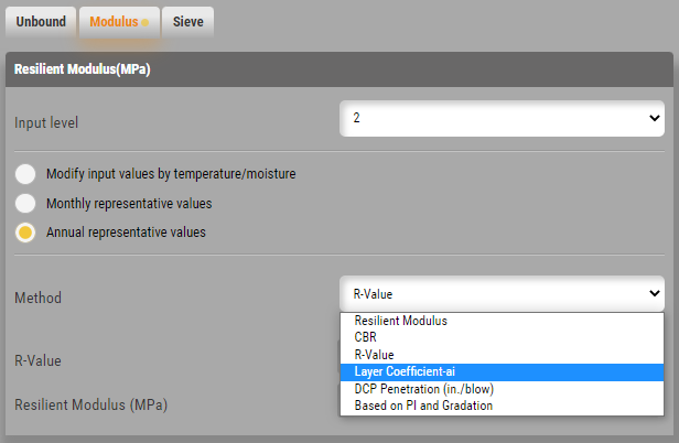
Figure 373: Subgrade Modulus

Aggregate Gradation and other engineering properties

The aggregate gradation dialog box allows you to define the particle size distribution, Atterberg limits, specific gravity, water content, maximum dry density, saturated hydraulic conductivity and the SWCC parameters of subgrade materials. A description of the available inputs are summarized below.

Sieve Size Table: This table allows you to define the percentage of subgrade material passing a variety of sieve sizes.
- Sieve Opening Size (in, mm): This column lists the applicable sieve sizes.
- Percent Passing: This column allows you to define the percentage of subgrade material passing a given sieve size. You are not required to define the percent passing for each sieve size. However, you are required to enter values for a minimum of 3 sieve sizes including No. 200 sieve.
- Liquid Limit This control allows you to define the liquid limit of the subgrade material.
- Plasticity Index: This control allows you to define the plasticity index for subgrade material.
- Is Layer Compacted?: Enable this control to indicate that the layer is compacted. Typically subgrade materials used in the base and subbase layers are compacted in place during construction. Disable this control to indicate that the layer is not compacted.
- Maximum dry unit weight (\(lb/ft^3\), \(kg/m^3\)): PMED internally computes the maximum dry unit weight of the subgrade material. This control allows you to override the internally computed value by enabling the check box. Click the check box to enable/disable this control.
- Saturated hydraulic conductivity (ft/hr, m/hr): PMED internally computes the saturated hydraulic conductivity of the subgrade material. This control allows you to override the internally computed value by enabling the check box. Click the check box to enable/disable this control.
- Specific gravity of solids: PMED internally computes the specific gravity of the subgrade material. This control allows you to override the internally computed value by enabling the check box. Click the check box to enable/disable this control.
- Optimum gravimetric water content (%): PMED internally computes the moisture content of the subgrade material at which maximum dry density is achieved. This control allows you to override the internally computed value by enabling the check box. Click the check box to enable/disable this control.
- User-defined Soil Water Characteristic Curve (SWCC): PMED internally computes the coefficients (af, bf, cf, and hr) of the soil water characteristic curve. This control allows you to override the internally computed value by enabling the check box. Click the check box to enable/disable this control.

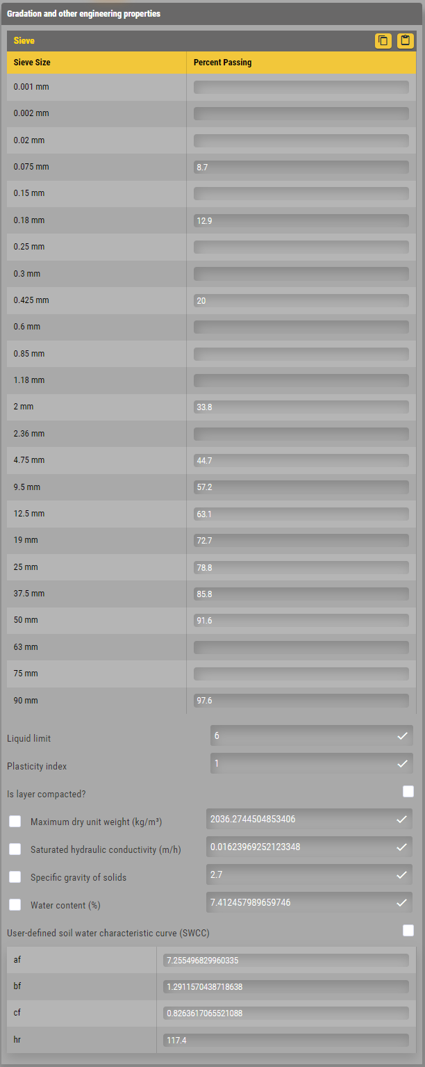
Figure 374: Subgrade Sieve

Note:
PMED internally computes the values of the following properties based on the inputs for Gradation, Liquid Limit, Plasticity Index and Is Layer Compacted. The computed values are based on the defaults initially displayed on the input screen. However, if you choose to modify the default values, you are required to click outside the input screen for the program to update the internally computed values.

Note:
Input compatibility: It is essential that the values entered for water content, maximum dry unit weight are compatible. If the value water content entered represents optimium conditions, then the maximum dry unit weight at optimum conditions should also be entered.

Bedrock

A bedrock layer, if present under an alignment, could have a significant impact on the pavement’s mechanistic responses and therefore need to be fully accounted for in design. This is especially true if backcalculation of layer moduli is adopted in rehabilitation design to characterize pavement materials. While the precise measure of the stiffness is seldom, if ever, warranted, any bedrock layer must be incorporated into the analysis.

Interface

Figure 375: Bedrock

Methods to Populate Inputs

Manual entry
Import from workspace library

Inputs

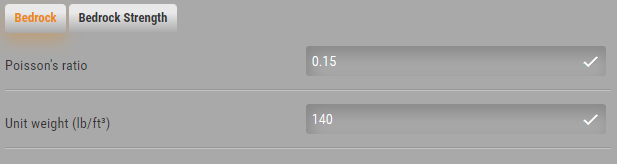
Bedrock

Layer thickness (in.): The program automatically defines the thickness of the bedrock layer as semi-infinite.
Poisson’s ratio: This control allows you to define the Poisson’s ratio of the bedrock material. PMED provides a default value of 0.15 for solid, massive and continuous bedrock material and 0.30 for highly fractured, weathered bedrock material.
Unit weight (pcf): This control allows you to define the weight per unit volume of the bedrock material. PMED uses a default value of 140 pcf.

Strength

Elastic/resilient Modulus (psi): This control allows you to define the modulus of the bedrock layer. PMED provides a default value of 750,000 psi for solid, massive and continuous bedrock material and 500,000 psi for highly fractured, weathered bedrock material.

Figure 376: Bedrock Strength

Design and Layer Properties

New Flexible Design Properties

AC Layer Design Properties

To access this component, create a design with the top layer having an AC layer, and select “Design Properties”.

AC Surface Shortwave Absorptivity: Defines the amount of available solar energy that is absorbed by the flexible pavement surface. PMED provides a default value of 0.85.
Layer Interface: Opens a table that allows you to define the friction at the interface of adjacent layers in the pavement system.
- Layer Name: Display name/ identifier you defined for the layer material type.
- Layer Type: Layer material type associated with the layer name.
- Interface Friction: Defines the friction of adjacent layers at their interface. Enter 0 for no friction (full slip condition), 1 for full friction (no slip), or between 0 and 1 for partial friction.

Endurance limit: Define the threshold tensile strain value (endurance limit) in microstrain.
Is endurance limit applied?: Determines whether or not you want to consider the endurance limit in the design analysis. Endurance limit is a threshold tensile strain value below which no load-related fatigue damage occurs in the AC layers. Select True to consider the endurance limit in the design analysis or False otherwise.
Uses multi-layer rutting calibration: Enables or disables multi-layer rutting calibration factors in the design.

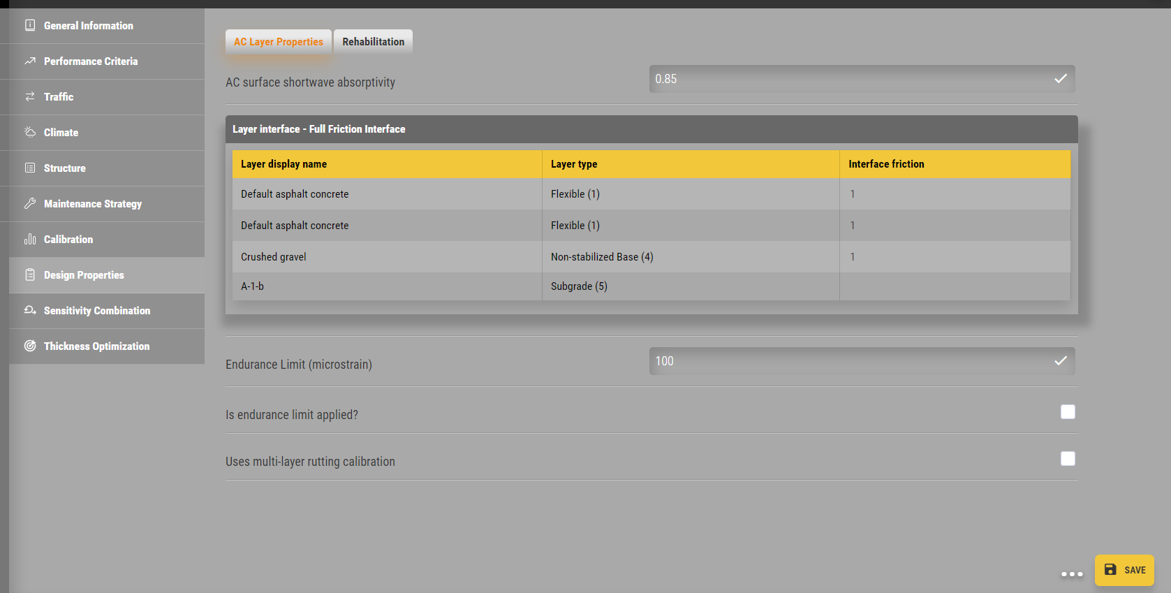
Figure 377: AC Layer Design Properties

JPCP Rehabilitation

This screen allows you to provide the required PMED inputs indicative of the existing level of distresses in a restoration or rehabilitation design.

The inputs enable PMED to estimate damage based on the condition of the existing pavement. The extent of repairs undertaken at the time of rehabilitation is used to adjust future performance predictions as needed.

Ways to Access this Interface

Open a rehabilitation project with a JPCP layer and select JPCP Rehabilitation in the Layer control.

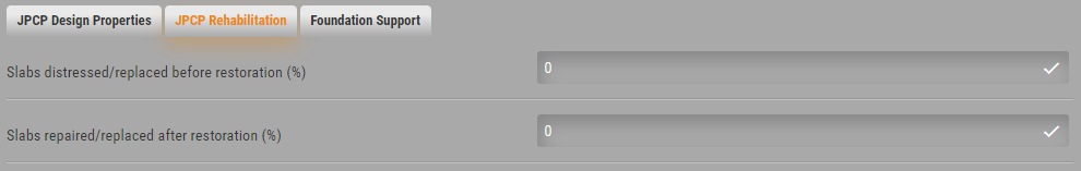
Figure 378: JPCP Rehabilitation

Ways to Enter Inputs

There are three methods for entering data for the PCC layer:

Manual entry
Import from file
Import from database

Populating the Inputs in this Interface

JPCP Rehabilitation

Slabs distressed/replaced before restoration (%): This control allows you to define the percentage of cracking in slabs before the restoration or rehabilitation. This is essentially the total percentage cracking in the slabs and includes all cracks that were previously.
Slabs repaired/replaced after restoration (%): This option allows you to define the percentage of slabs that were repaired during the restoration or rehabilitation process. The difference between the slabs distressed and slabs replaced is the percentage of slabs that are still cracked after restoration.

JPCP Design Properties

JPCP design features and construction practices influence long-term performance. The common design features that are considered by PMED include widened PCC slabs, joint spacing, shoulder type (tied vs untied PCC or asphalt concrete), presence and size of dowel bars used for transverse join tload transfer, dowel bar spacing, base type and erodibility, (chemically stabilized, asphalt stabilized, and non stabilized aggregate). Construction practices include PCC curing method (curing compound vs. wet curing), permanent curl/warp effective temperature difference in the PCC, PCC/base layer friction loss age, initial smoothness, and so on. Some of these design features and construction practices have been described in previous sections.

PCC surface shortwave absorptivity: This control allows you to define the fraction of solar energy (sunshine) at the PCC surface that is absorbed by the PCC. PMED presents a default value of 0.85. You can override this default.
Doweled joint spacing (ft): This control allows you to define the transverse joint load transfer mechanism.
- Dowel diameter (in.): This option allows you to define the diameter of the dowel bars used for load transfer across the transverse joint. A value of zero implies there are no dowel bars and load transfer is primarily through aggregate interlock.
- Dowel spacing (in.): This option allows you to define the center-to-center distance between adjacent dowel bars if used for load transfer across transverse joints.
- Is joint doweled?: This control allows you to select whether transverse joint load transfer mechanism is through the dowel bars:
  - True: Selecting this option implies transverse joint load transfer mechanism is through dowel bars.
  - False: Selecting this option implies transverse joint load transfer mechanism is through aggregate interlock only.

Erodibility index: This control allows you to select the resistance of the base course to erosion, using an index on a scale of 1 to 5. Material erosion resistance is determined both by its strength and durability. PMED allows you to select one of the following options:
- Extremely erosion resistant: Select an erodibility index of 1 for extremely erosion resistant base materials such as asphalt concrete and lean concrete materials.
- Very erosion resistant: Select an erodibility index of 2 for very erosion resistant base materials such as asphalt treated and cement treated materials.
- Erosion resistant: Select an erodibility index of 3 for erosion resistant base materials.
- Fairly erodible: Select an erodibility index of 4 for fairly erodible base materials such as weakly stabilized aggregate materials and subgrade soils.
- Very erodible: Select an erodibility index of 5 for very erodible base materials such as unstabilized subgrade soils.

PCC-base contact friction: The interface between the underlying base and PCC slab is modeled with or without full friction for JPCP design. PMED allows you to (1) determine whether or not the PCC slab/base interface has full friction at construction and (2) how long full friction will be available at the interface if present after construction. This control displays options available for modeling PCC slab/base interface condition.
- Months until friction loss: This option allows you to define the number of months after which full friction at the PCC slab/base interface is lost. The AASHTO Manual of Practice presents recommendations according to base material type. PMED allows for a range of 0 to 1200 months.
- Unbounded JPCP: This option allows you to select whether or not there is full friction at the PCC slab/base interface after construction. PMED allows you to select one of the following options:
  - True: Selecting this option implies there is full friction at the PCC slab/base interface after friction.
  - False: selecting this option implies there is relatively little to no friction at the PCC slab/base interface after friction.

PCC joint spacing (ft): This control allows you to define whether transverse joints of the trial design are uniformly or randomly spaced.
- Is joint spacing random? This control allows you to define whether transverse joints are uniformly spaced or randomly spaced. PMED allows for the following options:
- True: Selecting this option implies transverse joint are randomly spaced.
  - Spacing of joint 1: This option allows you to define the length of the first PCC slab.
  - Spacing of joint 2: This option allows you to define the length of the second PCC slab.
  - Spacing of joint 3: This option allows you to define the length of the third PCC slab.
  - Spacing of joint 4: This option allows you to define the length of the fourth PCC slab.
- False: Selecting this option implies transverse joint are uniformly spaced.
- Joint spacing: This option allows you to define average length of all the PCC slabs.

Permanent curl/warp effective temperature difference (deg F): This input describes the combined effect of (1) PCC built-in temperature gradient at time of set, (2) effective gradient of moisture warping in the PCC (dry on top and wet on bottom), (3) long term creep of the PCC slab, and (4) settlement of the PCC into the base. It is defined in terms of equivalent temperature difference. PMED presents the default value of -10 °F which was established as optimum to minimize error between measured and predicted cracking and measured and predicted faulting during the national calibration.
Sealant type: This control allows you to select the sealant type applied at the transverse joints. PMED allows you to choose from the following sealant types: preformed, liquid, and silicone.

Note:
Sealant type is an input to the JPCP transverse joint spalling model. Spalling is a key input for JPCP smoothness prediction.

Tied shoulders: This control allows you to select whether or not to use tied PCC shoulders. PMED allows you to select one of the following options:
- True: Selecting this option implies the use of tied PCC shoulders.
- False: Selecting this option implies the use of other shoulder types such as PCC (without tiebars), asphalt concrete, or gravel shoulders.
- Load transfer efficiency (%): This option allows you to define the long-term or terminal deflection LTE at the lane (PCC outer lane slab) to PCC shoulder longitudinal joint. PMED provides a default value of 50 percent. Typical long-term LTE are 50 to 70 percent for monolithically constructed tied PCC shoulder and 30 to 50 percent for separately constructed tied PCC shoulder.

Widened slab: This control displays if the PCC slabs are widened. Note that the typical JPCP PCC slab width is 12-ft.
- Is slab widened? This control allows you to select whether or not the JPCP PCC slab width is widened. PMED allows you to select one of the following options:
  - True: Selecting this option implies that the PCC slabs are widened (slab width is greater than 12-ft, typically 13- or 14-ft)
  - False: Selecting this option implies that the PCC slabs are not widened (slab width is 12-ft)
- Slab width (ft.): This option allows you to define the slab width. Note slab width is defined only when widened PCC slab option is applied. Otherwise, PMED assumes a standard 12-ft slab width.

PCC-base contact friction: The interface between the underlying base and PCC slab is modeled with or without full friction for JPCP design. PMED allows you to (1) determine whether or not the PCC slab/base interface has full friction at construction and (2) how long full friction will be available at the interface if present after construction. This control displays options available for modeling PCC slab/base interface condition.
PCC-Base full-friction contact: This option allows you to select whether or not there is full friction at the PCC slab/base interface after construction. PMED allows you to select one of the following options:
- True: Selecting this option implies there is full friction at the PCC slab/base interface after friction.
- False: selecting this option implies there is relatively little to no friction at the PCC slab/base interface after friction.

Months until friction loss: This option allows you to define the number of months after which full friction at the PCC slab/base interface is lost. The AASHTO Manual of Practice presents recommendations according to base material type. PMED allows for a range of 0 to 1200 months.

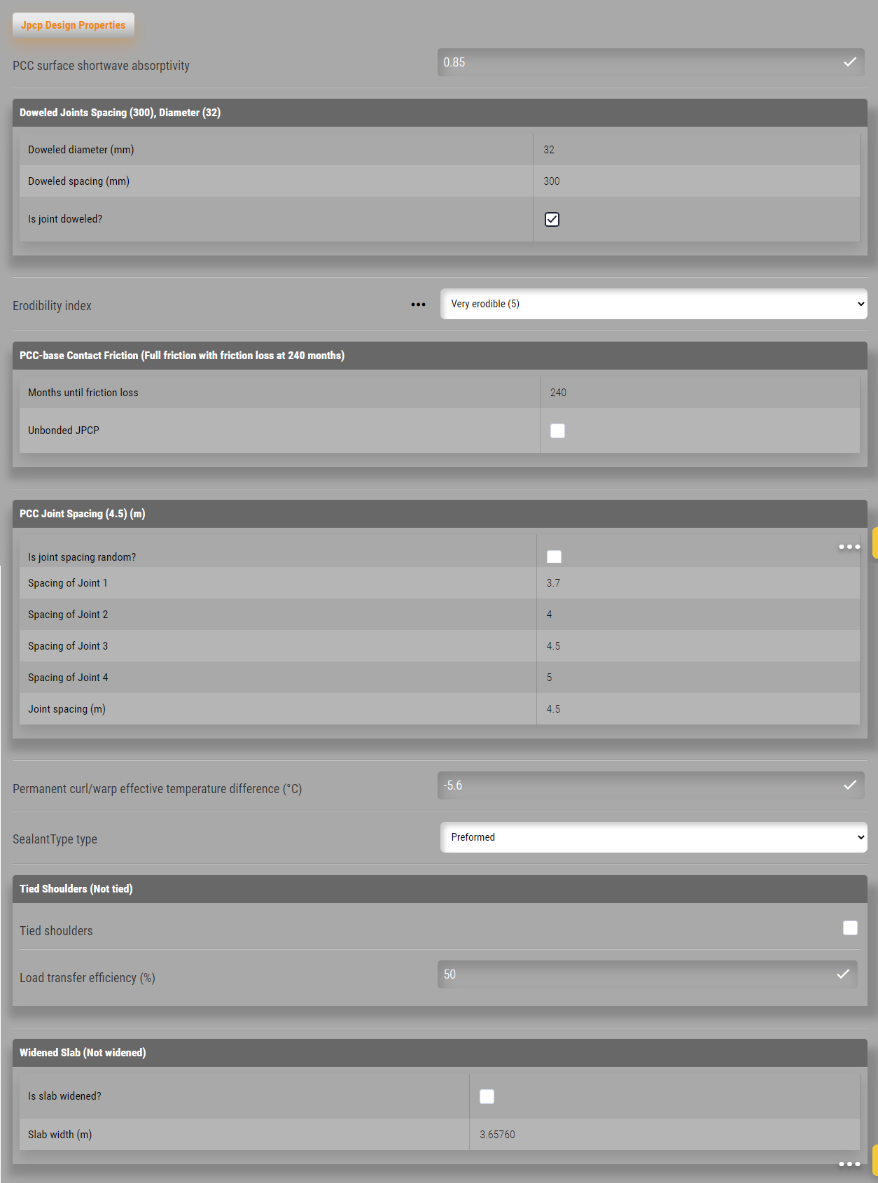
Figure 379: JPCP Design Properties

Foundation Support

Modulus of subgrade reaction, or k-value, is a soil support parameter. The static k-value is determined from the plate load test and is a measure of the pressure applied on the soil for a unit deformation monitored using a standard size plate. Dynamic k-value is determined through deflection testing and backcalculation. PMED requires dynamic k-value.

Ways to Access this Interface

Open a rehabilitation project with a foundation layer and select Foundation Support in the Layer control.

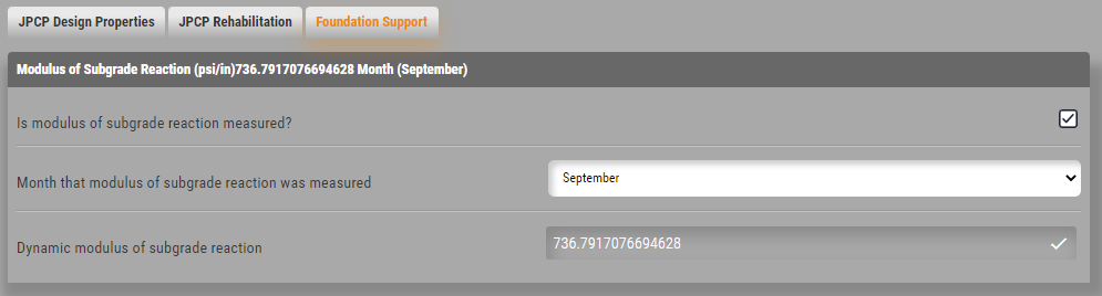
Figure 380: Foundation Support

Ways to Enter Inputs

There are three methods for entering data for the sandwiched granular layer:

• Manual entry • Import from file • Import from database

Modulus of Subgrade Reaction

• Modulus of subgrade reaction: This control displays whether the modulus of subgrade reaction is calculated internally by PMED or user-defined.

• Is modulus of subgrade reaction measure?: Select True to define the modulus of subgrade reaction (k-value) and the month of the year it was measured. Select False to allow PMED to compute this value.

• Dynamic modulus of subgrade reaction (psi/in.): This control allows you to define the dynamic k-value.

• Month modulus of subgrade reaction measured: This control allows you to define the month of the year when the dynamic k-value was measured.

Structural Response

PMED’s structural model analyzes pavement structure, accounts for discontinuities in that structure, and analyzes the effects of environment and traffic on that structure.

PMED produces the structure response outputs as intermediate files:

Vertical compressive strain values are stored in the file “_VertStrain.txt”.
Horizontal tensile strain values are stored in the file “_TensStrain.txt” The information contained in both files is as follows:
Month
SubMonth
SubSeason
Axle Number
AC Modulus
Load location
Analysis location
Strain (either vertical compression or horizontal tension) These files are located in the project folder where is the project file is stored.

PMED produces several intermediate files that contain a wide range of calculated output parameters. The contents of some of these files are described at http://www.me-design.com.

Calibration Factors

Calibration Factors for AC|JPCP include

AC Cracking-Bottom Up

AC Cracking C1 Bottom: Asphalt concrete bottom-up cracking value for C1.
AC Cracking C2 Bottom: The asphalt concrete bottom-up cracking value for C2 is provided for three different pavement thicknesses < 5in, 5in < thickness (hac) < 12in, and > 12in.
AC Cracking C3 Bottom: Asphalt concrete bottom-up cracking value for C3.
AC Cracking Bottom Standard Deviation: Dispersion from the average bottom-up cracking value for asphalt concrete.

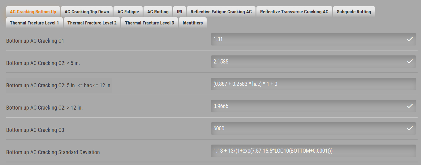
Figure 381: AC Cracking Bottom-up

AC Cracking-Top Down

AC Top-Down AC Cracking C1: Asphalt concrete top-down cracking value for C1.
AC Top-Down AC Cracking C2: Asphalt concrete top-down cracking value for C2.
AC Top-Down AC Cracking C3: Asphalt concrete top-down cracking value for C3.
AC Top-Down AC Cracking kL1: Asphalt concrete top-down cracking value for kL1.
AC Top-Down AC Cracking kL2: Asphalt concrete top-down cracking value for kL2.
AC Top-Down AC Cracking kL3: Asphalt concrete top-down cracking value for kL3.
AC Top-Down AC Cracking kL4: Asphalt concrete top-down cracking value for kL4.
AC Top-Down AC Cracking kL5: Asphalt concrete top-down cracking value for kL5.
AC Top-Down Cracking Standard Deviation: Dispersion from the average top-down cracking value for asphalt concrete.

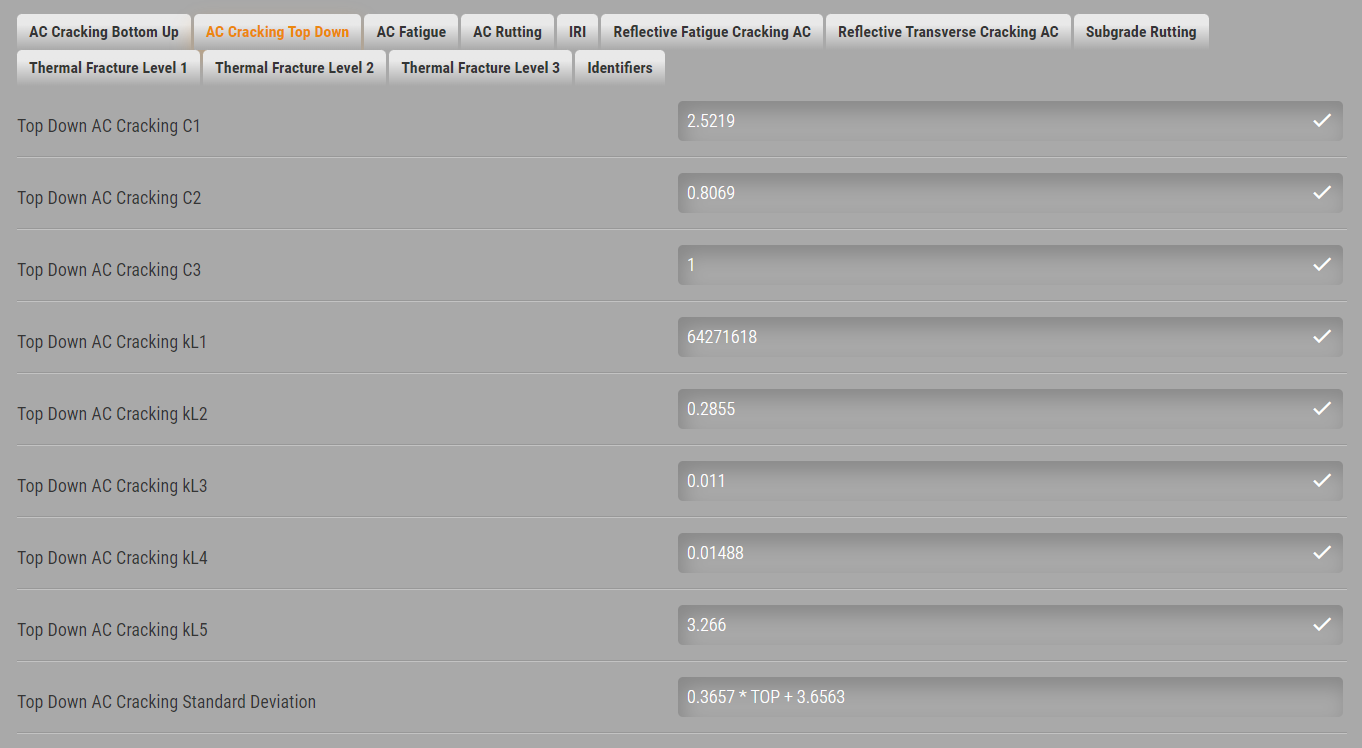
Figure 382: AC Cracking Top-down

AC Fatigue

AC Fatigue K1: Asphalt concrete repetitive-loading or fatigue damage value for K1.
AC Fatigue K2: Asphalt concrete repetitive-loading or fatigue damage value for K2.
AC Fatigue K3: Asphalt concrete repetitive-loading or fatigue damage value for K3.
AC Fatigue BF1: The asphalt concrete repetitive-loading or fatigue damage value for BF1 is provided at three pavement thicknesses, < 5in, 5in < thickness (hac) < 12in, and > 12in.
AC Fatigue BF2: Asphalt concrete repetitive-loading or fatigue damage value for BF2.
AC Fatigue BF3: Asphalt concrete repetitive-loading or fatigue damage value for BF3.

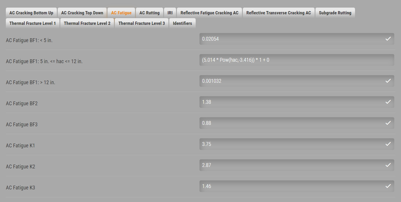
Figure 383: AC Fatigue

AC Rutting

AC rutting calibration factors can be used in two ways:

Single-Layer AC Rutting Calibration You can assume the same set of calibration factors for all asphalt layers by setting Uses multi-layer rutting calibration under AC Layer Properties as “False”.

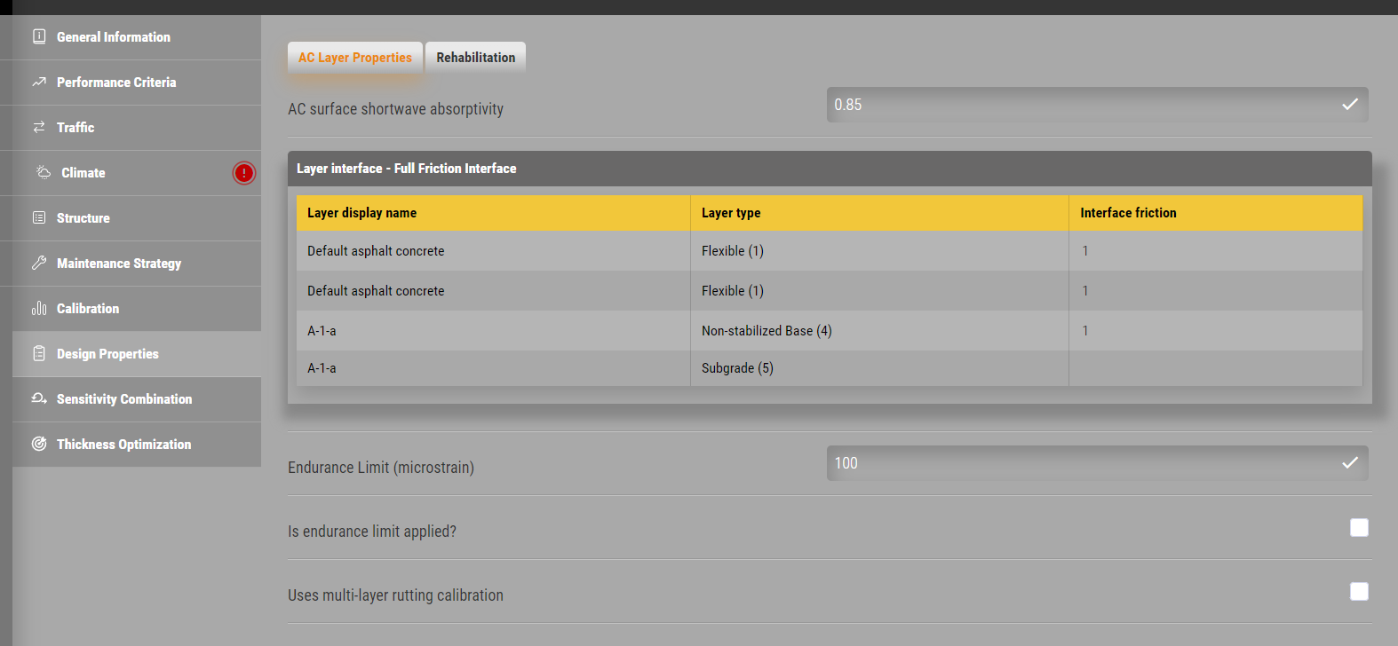
Figure 384: AC Layer Properties

AC rutting calibration factors include:

AC Rutting BR1: Asphalt concrete longitudinal depression (wearing-away) value for BR1.
AC Rutting BR2: Asphalt concrete longitudinal depression (wearing-away) value for BR2.
AC Rutting BR3: Asphalt concrete longitudinal depression (wearing-away) value for BR3.
AC Rutting K1: Asphalt concrete longitudinal depression (wearing-away) value for K1.
AC Rutting K2: Asphalt concrete longitudinal depression (wearing-away) value for K2.
AC Rutting K3: Asphalt concrete longitudinal depression (wearing-away) value for K3.
AC Rutting Standard Deviation: Dispersion from the average longitudinal depression (wearing-away) value for asphalt concrete.

Multi-Layer AC Rutting Calibration You can assume different sets of calibration factors for each asphalt layer by setting Uses multi-layer rutting calibration under AC Layer Properties as “True”. You can add up to three asphalt layers for new flexible pavement; therefore, up to three sets of rutting calibration factors can be used.

Flexible IRI Calibration Factors

IRI Flexible C1: Flexible pavement international roughness index (IRI) value for C1, which is the contribution from total rutting.
IRI Flexible C2: Flexible pavement IRI value for C2, which is the contribution from fatigue cracking (both top-down and bottom-up).
IRI Flexible C3: Flexible pavement IRI value for C3, which is the contribution from thermal cracking.
IRI Flexible C4: Flexible pavement IRI value for C4, which is the contribution from site factor.

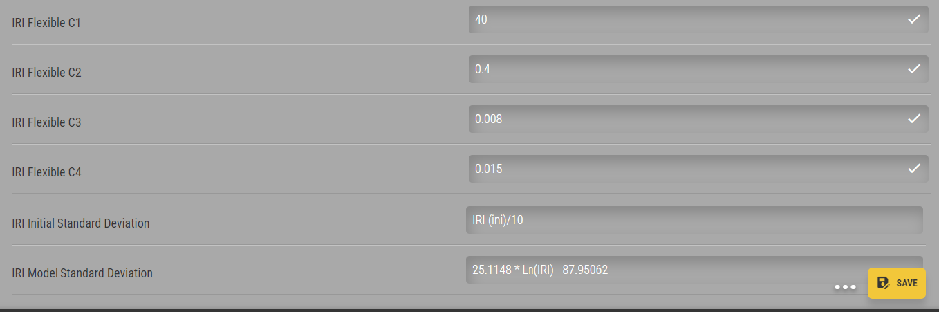
Figure 385: IRI Flexible

IRI Flexible Over PCC

IRI Flexible Over PCC C1: Flexible over PCC pavement IRI value for C1.
IRI Flexible Over PCC C2: Flexible over PCC pavement IRI value for C2.
IRI Flexible Over PCC C3: Flexible over PCC pavement IRI value for C3.
IRI Flexible Over PCC C4: Flexible over PCC pavement IRI value for C4.

Figure 386: IRI Flexible

Reflective Fatigue Cracking

Reflective Fatigue Cracking AC C1: Reflective fatigue cracking C1
Reflective Fatigue Cracking AC C2: Reflective fatigue cracking C2
Reflective Fatigue Cracking AC C3: Reflective fatigue cracking C3
Reflective Fatigue Cracking AC C4: Reflective fatigue cracking C4
Reflective Fatigue Cracking AC C5: Reflective fatigue cracking C5
Reflective Fatigue Cracking AC K1: Reflective fatigue cracking K1
Reflective Fatigue Cracking AC K2: Reflective fatigue cracking K2
Reflective Fatigue Cracking AC K3: Reflective fatigue cracking K3
Reflective Fatigue Cracking AC Standard Deviation: Reflective fatigue cracking standard deviation equation

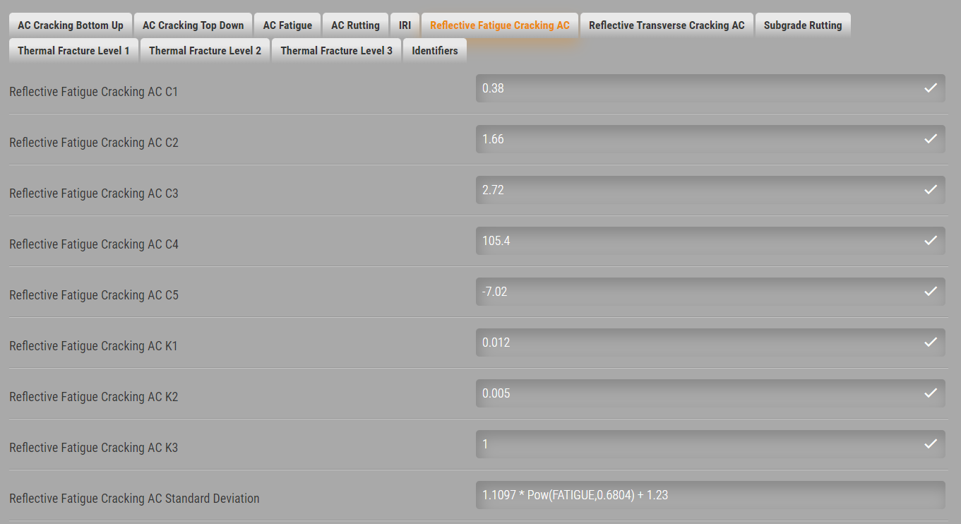
Figure 387: Reflective Fatigue Cracking AC

Reflective Transverse Cracking

Reflective Transverse Cracking AC C1: Reflective fatigue cracking C1
Reflective Transverse Cracking AC C2: Reflective fatigue cracking C2
Reflective Transverse Cracking AC C3: Reflective fatigue cracking C3
Reflective Transverse Cracking AC C4: Reflective fatigue cracking C4
Reflective Transverse Cracking AC C5: Reflective fatigue cracking C5
Reflective Transverse Cracking AC K1: Reflective fatigue cracking K1
Reflective Transverse Cracking AC K2: Reflective fatigue cracking K2
Reflective Transverse Cracking AC K3: Reflective fatigue cracking K3
Reflective Transverse Cracking AC Standard Deviation: Reflective fatigue cracking standard deviation equation

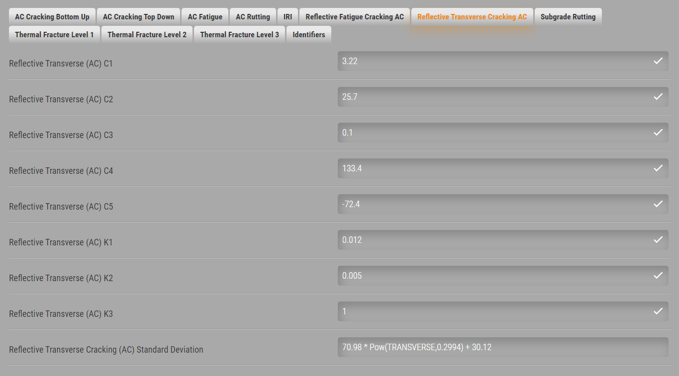
Figure 388: Reflective Transverse Cracking AC

Subgrade Rutting

Granular Base Rutting BS1: Subgrade longitudinal depression (wearing-away) value for BS1.
Granular Base Rutting K1: Subgrade longitudinal depression (wearing-away) value for K1.
Granular Base Rutting Standard Deviation: Dispersion from the average longitudinal depression (wearing-away) value for subgrade (Fine).
Subgrade A-3 Rutting K1: Subgrade longitudinal depression (wearing-away) value for K1 and A-3 subgrade.
Subgrade Coarse Grained Rutting K1: Subgrade (coarse) longitudinal depression (wearing-away) value for K1.
Subgrade Fine Grained Rutting K1: Subgrade (fine) longitudinal depression (wearing-away) value for K1.
Subgrade Rutting BS1: Granular base longitudinal depression (wearing-away) value for BS1.
Subgrade Rutting Standard Deviation: Dispersion from the average longitudinal depression (wearing-away) value for granular base.

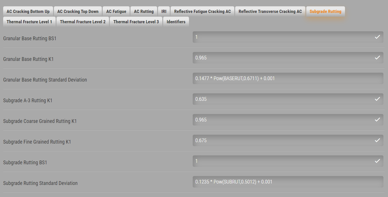
Figure 389: Subgrade Rutting

PCC Cracking

PCC Cracking C1: JPCP repetitive-loading or fatigue damage value for C1.
PCC Cracking C2: JPCP repetitive-loading or fatigue damage value for C2.
PCC Cracking C4: JPCP cracking value for C4.
PCC Cracking C5: JPCP cracking value for C5.
PCC Reliability Cracking Standard Deviation: Dispersion from the average cracking value for JPCP.

Figure 390: PCC Cracking